Structure Learning via Independence Testing
(c) David Merrell 2018
We're interested in learning a graph structure over gene expression variables.
The structure shared by a set of random variables can be estimated efficiently under these assumptions:
- The variables' joint distribution is log-linear.
- The joint distribution encodes pairwise interactions---no higher-order interactions.
I.e., the joint distribution looks like this:
$$ P(x) \propto \exp \left[ \sum_i \phi_i f_i(x_i) + \sum_{ij} \theta_{ij} f_{ij}(x_i, x_j) \right]$$In the special case of a multivariate Gaussian distribution $\mathcal{N}(\mu, \Sigma)$, structure learning consists of figuring out which entries of its precision matrix $P = \Sigma^{-1}$ are zero. In this case, it turns out that structure learning reduces to a linear regression task. We can even enforce sparsity by adding an $L_1$ regularizer. (If we don't do that, then we'll probably learn a fully connected structure; very unhelpful).
The assumption of pairwise interactions is very strong and will probably not hold for complicated domains like cellular biology, where variables are highly coupled. We'll demonstrate the method for MNIST images and then see if it does anything useful for gene expression.
# Load packages
from keras.datasets.mnist import load_data
from sklearn.preprocessing import StandardScaler
from sklearn.linear_model import Lasso
import matplotlib.pyplot as plt
import numpy as np
import pandas as pd
Estimating the Precision Matrix
We build some machinery for estimating a precision matrix from data.
Strictly speaking, we aren't going to bother estimating the precision matrix itself; we're just going to figure out which of its entries we can afford to set to zero. We're looking for sparse structure.
When we're dealing with images (like MNIST), we would expect to recover a grid-like structure: the precision matrix should be nonzero only for pixels that are near each other. We'll see if that is indeed the case.
For other kinds of data (e.g. gene expression), it's unclear what kind of structure we'd find. We'll give it a try and see what happens!
def gauss_sparse_precision(X, alpha=1.0):
    """
    Receives 2D array X (rows are instances; columns are features) and
    returns a binary matrix; entries are zero where the data's precision matrix is zero,
    and binary otherwise.
    """

    result = np.zeros((X.shape[-1], X.shape[-1]))

    for i in range(X.shape[-1]):

        #if i % 10 == 0:
        #    print("Estimating row {}.".format(i))

        y_col = X[:,i]
        X_cols = np.concatenate([X[:,:i], X[:,(i+1):]], axis=-1)

        reg = Lasso(fit_intercept=False, alpha=alpha)
        reg.fit(X_cols, y_col)

        result[i,:i] = reg.coef_[:i]
        result[i,(i+1):] = reg.coef_[i:]


    return result
def estimate_precision_row(args, alpha=1.0):
    """
    Estimate the ith row of X's precision matrix.
    (kind of; we're only interested in finding zero-entries after enforcing sparsity.)
    """
    X = args[0]
    i = args[1]
    alpha=args[2]

    print("Estimating {}th row!".format(i))

    result = np.zeros((X.shape[-1],))

    y_col = X[:,i]
    X_cols = np.concatenate([X[:,:i], X[:,(i+1):]], axis=-1)
    reg = Lasso(fit_intercept=False, alpha=alpha)
    reg.fit(X_cols, y_col)

    result[:i] = reg.coef_[:i]
    result[(i+1):] =reg.coef_[i:]

    return result
Example: Finding Structure in MNIST
For illustration, we'll first apply gauss_sparse_precision to a subset of the MNIST data.
This will inform our intuitions when we move on to the LINCS gene expression dataset.
Prepare MNIST Data
Note that we standardize the data. Standardizing is benign and even desirable for independence testing. It won't make any of the precision matrix's zero entries non-zero, or vice-versa. Meanwhile, it will also make our regression tasks better-conditioned (and hence faster to solve).
(train_X, train_y), (test_X, test_y) = load_data()
X = np.concatenate([train_X, test_X], axis=0)
X_flat = np.reshape(X,(X.shape[0],X.shape[1]*X.shape[2]))

y = np.concatenate([train_y, test_y], axis=0)
print("Instance Shape: {}\tLabels: {}".format(X_flat.shape[1:], np.unique(y)))

std = StandardScaler()
X_flat = std.fit_transform(X_flat,y)
plt.imshow(X[777,:,:], cmap="Greys")
plt.show()

Learning a graph for MNIST
It turns out that this is computationally expensive! It takes my laptop about 5 minutes to do all of the requisite regression tasks.
When we move to a larger dataset (i.e. LINCS), we'll need to do some multiprocessing. I'd parallelize these regression tasks right here, but I'm writing this notebook on my wimpy laptop.
mat = gauss_sparse_precision(X_flat[:1000,:], alpha=0.25)
We binarize the precision matrix according to a threshold rule.
binmat = (np.abs(mat) >= 1e-5).astype(int)
We plot its entries; the diagonal-like pattern suggests that we have sparse structure!
plt.figure(figsize=(10,10))
plt.imshow(binmat,cmap="binary")
plt.show()

We've visualized the graph's adjacency matrix; now let's visualize the graph in pixel space!
The structure ought to resemble the original pixel grid.
coords_X, coords_Y = np.meshgrid(range(28), range(28))
flat_coords_X = np.reshape(coords_X, 784)
flat_coords_Y = np.reshape(coords_Y, 784)
coords = np.transpose([flat_coords_X,flat_coords_Y])
def plot_graph(v_coords, adj_mat, **kwargs):
    for i in range(adj_mat.shape[0]):
        for j in range(i):
            if adj_mat[i,j] != 0:
                plt.plot([v_coords[i,0],v_coords[j,0]], [v_coords[i,1], v_coords[j,1]], **kwargs)
plt.figure(figsize=(10,10))
plot_graph(coords, binmat)
plt.show()

Very satisfying: the method recovered a lot of the grid structure that we hoped it would.
It's not perfect---there are some spurious connections, and a lot of missing connections in the corners (where the pixels were uninformative). But suppose we had started without any knowledge that this was image data; this method would have captured much of the pixel topology on its own!
Finding Structure in LINCS
Following a similar process for the LINCS landmark gene expression data yields the following matrix of dependencies:
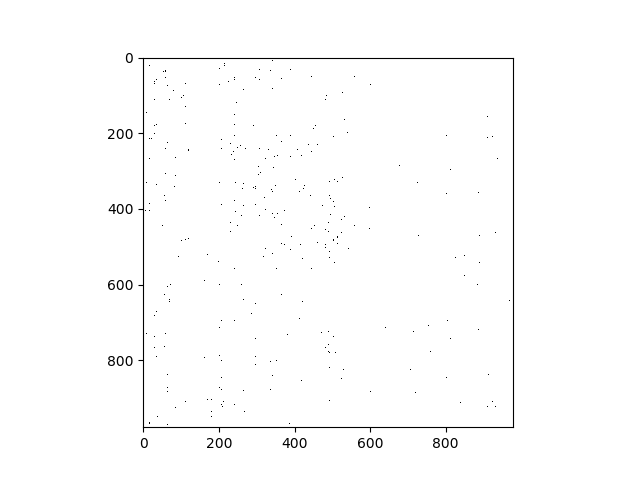
(I'm just displaying the results; I did the computation in parallel on a remote server.)
(This seems too sparse. Decreasing the Lasso coefficient may produce more edges, but more of them may be spurious.)
I used Networkx and Cytoscape to display the graph:
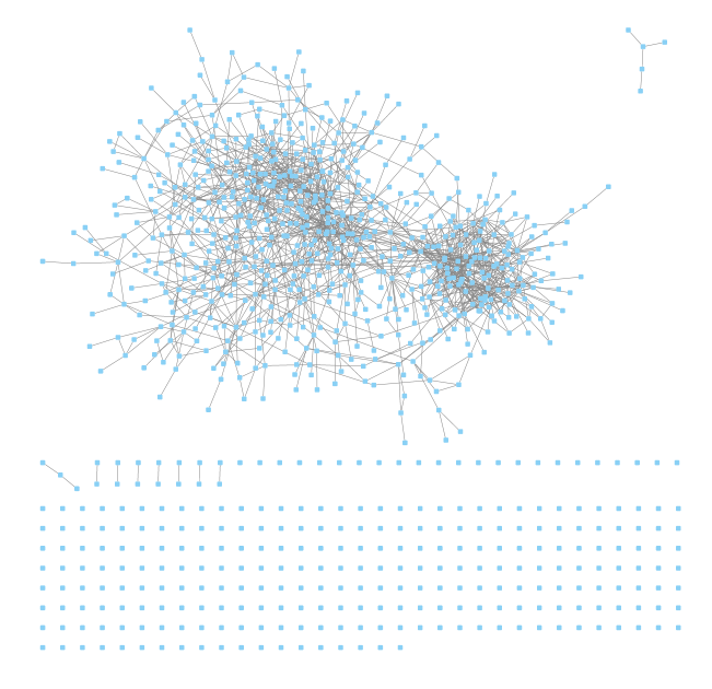
Observations:
- There appear to be two large clusters of highly related genes. We'll have to see whether they have biological meaning.
- There are several genes disconnected from the graph. Apparently Lasso eliminated all of their dependencies!(similar to the uninformative edge pixels from the MNIST example).
To do:
- Need to label the nodes with gene names. Then we'll be able to judge the biological properties of this graph.
- Are the learned graphs stable? I.e., do they vary much with randomness in the training set? This could be evaluated by learning a graph on disjoint subsets of the instances, and seeing how much the graphs vary.