A less-bad blog post about transformers

This is the second post in a series!

I recommend reading the first post (“A less-bad blog post about attention mechanisms”) before reading this one. It explains important prerequisite concepts. For example, “self-attention” and “multi-head attention.”

Why I’m writing this

I suspect “Attention is All You Need” (AIAYN) was written with a very specific audience in mind. I don’t think it actually explains transformers very well to a general ML audience.

As a single example, consider this graphic from the original AIAYN paper:

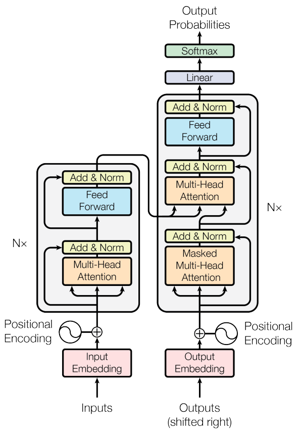
This was incomprehensible to me when I first tried reading AIAYN.

• What’s being stacked N times? And in what fashion? How do connections work between stacked units on the left and right?
• Why is there an arrow from outputs into the network?
• What does it mean that the outputs are “shifted right?”
• Why are there “outputs” in the lower right and “output probabilities” in the upper right?

Despite its (arguable) lack of clarity, this same image is copied and pasted into practically every blog post about transformers. The typical blogger then proceeds to “explain” it by parroting the same explanation given in AIAYN. It’s as though the bloggers only have a superficial understanding of the concepts in AIAYN, or haven’t thought carefully about how to explain them.

This post aims to do a less-bad job of explaining transformers to a broad ML audience.

A gradual explanation of the transformer architecture

We’ll start with a 10,000-foot view of the transformer and gradually zoom in, focusing on important details as appropriate.

Broad brush strokes

Some important big-picture things to understand about the transformer architecture:

• The transformer is a sequence-to-sequence model.
  • That is, it receives a sequence \(x_1, x_2, \ldots, x_M \) as input and produces a new sequence \(y_1, y_2, \ldots, y_N\) as output.
  • Concretely, AIAYN presents the transformer as a model for translating text from one language to another (like in Google Translate).
  • Whenever appropriate, we’ll focus on concrete examples from text translation. But keep in mind that the architecture may accommodate a much broader class of tasks.
• The transformer has two primary components: an encoder and a decoder.
  • The encoder receives an input sequence and transforms it into a latent representation. The idea is that this latent representation encodes the input in some informative way.
  • The decoder receives the latent representation and transforms it into a useful output. (It operates differently from your typical decoder, though—pay special attention to the graphics in this post.)
• The transformer is autoregressive. That is:
  • it generates the output sequence one item at a time; and
  • each new item in the output sequence is a function of the previous items.
  • The output sequence terminates when a special “end token” is generated.

The situation is captured in this graphic:

The transformer’s encoder receives the input sequence \(x_1, x_2, \ldots, x_M \) and computes a latent representation for it. This latent representation gets passed to the decoder.

In this scenario, the transformer has already generated the first \(t \) items in the output sequence—\(y_1, y_2, \ldots, y_t\). The decoder generates \(y_{t+1}\) as a function of (i) the latent representation and (ii) the first \(t\) items. Finally, \(y_{t+1} \) is appended to the output sequence and the process repeats. Note that the latent representation remains the same while the output items are being generated. That is, the latent representation only needs to be computed once for the input sequence.

Layers of the model

It’s time to reveal more details. The encoder and decoder are each composed of layers. For example, In AIAYN they both contain \(K = 6\) layers.

The layers in the encoder all have identical architecture, though their weights are allowed to differ. The same applies to the decoder: its layers have identical architecture but differing weights. We’ll discuss the encoder and decoder layers later in much more detail.

Here’s the graphic again, updated to show the layers:

The encoder’s final layer produces the latent representation. Interestingly, it passes the latent representation to every layer of the decoder. This ensures that the input sequence thoroughly “informs” the generation of the next item in the output sequence.

Here’s an important detail that isn’t captured in the graphic: the latent representation is actually a collection of \(M\) vectors; i.e., a collection as long as the original input sequence. And this collection of \(M\) vectors gets passed to each layer of the decoder. Just imagine that each of the edges from encoder to decoder is actually a collection of \(M\) edges.

Notice that the next output item, \( y_{t+1} \), is a function of the outputs of the final decoder layer. A more complete explanation is that \(y_{t+1} \) is computed via a linear function followed by a softmax. Importantly, the transformer assumes you have a fixed-size vocabulary of possible output items (e.g., the 10,000 most common English words). The decoder selects the next token by (i) assigning probabilities to the vocabulary items and (ii) choosing the most probable item. (This amounts to a one-hot encoding of \(y_{t+1} \)—which was a point of confusion for me since one-hot encodings are not used anywhere else in the model.)

Much of the credit for this graphic goes to Jay Alammar’s “The Illustrated Transformer,” one of the few blog posts I found useful for understanding transformers. Before reading his post I found it difficult to understand the connections between the encoder and decoder.

Encoder layers and sublayers

TODO

• Self-attention layer
• Fully connected, position-wise neural network
• Layer norm
• Residual connections

Decoder layers and sublayers

TODO

• Three sublayers, rather than two. Same layer norms and residual connections as before.
• First sublayer: masked self-attention
• Second sublayer: self-attention, including the input’s latent representation
• Third layer: fully connected, position-wise neural network

Input representations

TODO

• Positional encoding
• Connection to Fourier series
• This is one of the very few ways sequence information is preserved in the input.

Beyond sequence-to-sequence tasks

The transformer described in AIAYN has very few attributes tailoring it specifically to sequence-to-sequence tasks:

• The positional encoding
• The masked self-attention in the decoder
• The autoregressive generative process

With the right modification, it can be quite serviceable for other classes of tasks.

• Domain-appropriate encodings can encourage relevant pairs of inputs tend to pay attention to each other.
• The attention-masking can easily be removed from the decoder, if it’s not appropriate for a given application domain.
• It’s not too difficult to define autoregressive processes for non-sequence data.

Other reading

• Attention is All You Need (Vaswani et al. 2017)
• The Illustrated Transformer (Jay Alammar)
• The Transformer Family (Lilian Weng)
• On Layer Normalization in the Transformer Architecture (Xiong et al 2020)

\( \blacksquare\)